Storage Engine

The 0.9 line of InfluxDB used BoltDB as the underlying storage engine. This writeup is about the experimental version of the Time Structured Merge Tree storage engine that was released in 0.9.5. There may be small discrepancies between the current implementation of TSM and this document.

See the blog post announcement about the storage engine here.

The new InfluxDB storage engine: from LSM Tree to B+Tree and back again to create the Time Structured Merge Tree

The properties of the time series data use case make it challenging for many existing storage engines. Over the course of InfluxDB’s development we’ve tried a few of the more popular options. We started with LevelDB, an engine based on LSM Trees, which are optimized for write throughput. After that we tried BoltDB, an engine based on a memory mapped B+Tree, which is optimized for reads. Finally, we ended up building our own storage engine that is similar in many ways to LSM Trees.

With our new storage engine we were able to achieve up to a 45x reduction in disk space usage from our B+Tree setup with even greater write throughput and compression than what we saw with LevelDB and its variants. Using batched writes, we were able to insert more than 300,000 points per second on a c3.8xlarge instance in AWS. This post will cover the details of that evolution and end with an in-depth look at our new storage engine and its inner workings.

Properties of Time Series Data

The workload of time series data is quite different from normal database workloads. There are a number of factors that conspire to make it very difficult to get it to scale and perform well:

• Billions of individual data points
• High write throughput
• High read throughput
• Large deletes to free up disk space
• Mostly an insert/append workload, very few updates

The first and most obvious problem is one of scale. In DevOps, for instance, you can collect hundreds of millions or billions of unique data points every day.

To prove out the numbers, let’s say we have 200 VMs or servers running, with each server collecting an average of 100 measurements every 10 seconds. Given there are 86,400 seconds in a day, a single measurement will generate 8,640 points in a day, per server. That gives us a total of 200 * 100 * 8,640 = 172,800,000 individual data points per day. We find similar or larger numbers in sensor data use cases.

The volume of data means that the write throughput can be very high. We regularly get requests for setups than can handle hundreds of thousands of writes per second. I’ve talked to some larger companies that will only consider systems that can handle millions of writes per second.

At the same time, time series data can be a high read throughput use case. It’s true that if you’re tracking 700,000 unique metrics or time series, you can’t hope to visualize all of them, which is what leads many people to think that you don’t actually read most of the data that goes into the database. However, other than dashboards that people have up on their screens, there are automated systems for monitoring or combining the large volume of time series data with other types of data.

Inside InfluxDB, we have aggregates that can get calculated on the fly that can combine tens of thousands of time series into a single view. Each one of those queries does a read on each data point, which means that for InfluxDB, the read throughput is often many times higher than the write throughput.

Given that time series is a mostly an append only workload, you might think that it’s possible to get great performance on a B+Tree. Appends in the keyspace are efficient and you can achieve greater than 100,000 per second. However, we have those appends happening in individual time series. So the inserts end up looking more like random inserts than append only inserts.

One of the biggest problems we found with time series data is that it’s very common to delete all data after it gets past a certain age. The common pattern here is that you’ll have high precision data that is kept for a short period of time like a few hours or a few weeks. You’ll then downsample and aggregate that data into lower precision, which you’ll keep around for much longer.

The naive implementation would be to simply delete each record once it gets past its expiration time. However, that means that once you’re up to your window of retention, you’ll be doing just as many deletes as you do writes, which is something most storage engines aren’t designed for.

Let’s dig into the details of the two types of storage engines we tried and how these properties had a significant impact on our performance.

LevelDB and Log Structured Merge Trees

Two years ago when we started InfluxDB, we picked LevelDB as the storage engine because it was what we used for time series data storage for the product that was the precursor to InfluxDB. We knew that it had great properties for write throughput and everything seemed to just work.

LevelDB is an implementation of a Log Structured Merge Tree (or LSM Tree) that was built as an open source project at Google. It exposes an API for a key/value store where the key space is sorted. This last part is important for time series data as it would allow us to quickly go through ranges of time as long as the timestamp was in the key.

LSM Trees are based on a log that takes writes and two structures known as Mem Tables and SSTables. These tables represent the sorted keyspace. SSTables are read only files that continuously get replaced by other SSTables that merge inserts and updates into the keyspace.

The two biggest advantages that LevelDB had for us were high write throughput and built in compression. However, as we learned more about what people needed with time series data, we encountered a few insurmountable challenges.

The first problem we had was that LevelDB doesn’t support hot backups. If you want to do a safe backup of the database, you have to close it and then copy it. The LevelDB variants RocksDB and HyperLevelDB fix this problem so we could have moved to them, but there was another problem that was more pressing that we didn’t think could be solved with either of them.

We needed to give our users a way to automatically manage the data retention of their time series data. That meant that we’d have to do very large scale deletes. In LSM Trees a delete is as expensive, if not more so, than a write. A delete will write a new record known as a tombstone. After that queries will merge the result set with any tombstones to clear out the deletes. Later, a compaction will run that will remove the tombstone and the underlying record from the SSTable file.

To get around doing deletes, we split data across what we call shards, which are contiguous blocks of time. Shards would typically hold either a day or 7 days worth of data. Each shard mapped to an underlying LevelDB. This meant that we could drop an entire day of data by just closing out the database and removing the underlying files.

Users of RocksDB may at this point bring up a feature called ColumnFamilies. When putting time series data into Rocks, it’s common to split blocks of time into column families and then drop those when their time is up. It’s the same general idea that you create a separate area where you can just drop files instead of updating any indexes when you delete a large block of old data. Dropping a column family is a very efficient operation. However, column families are a fairly new feature and we had another use case for shards.

Organizing data into shards meant that it could be moved within a cluster without having to examine billions of keys. At the time of this writing I don’t think it’s possible to move a column family in one RocksDB to another. Old shards are typically cold for writes so moving them around would be cheap and easy and we’d have the added benefit of having a spot in the keyspace that is cold for writes so it would be easier to do consistency checks later.

The organization of data into shards worked great for a little while until a large amount of data went into InfluxDB. For our users that had 6 months or a year of data in large databases, they would run out of file handles. LevelDB splits the data out over many small files. Having dozens or hundreds of these databases open in a single process ended up creating a big problem. It’s not something we found with a large number of users, but for anyone that was stressing the database to its limits, they were hitting this problem and we had no fix for it. There were simply too many file handles open.

BoltDB and mmap B+Trees

After struggling with LevelDB and its variants for a year we decided to move over to BoltDB, a pure Golang database heavily inspired by LMDB, a mmap B+Tree database written in C. It has the same API semantics as LevelDB: a key value store where the keyspace is ordered. Many of our users were surprised about this move after we posted some early testing results of the LevelDB variants vs. LMDB (a mmap B+Tree) that showed RocksDB as the best performer.

However, there were other considerations that went into this decision outside of the pure write performance. At this point our most important goal was to get to something stable that could be run in production and backed up. BoltDB also had the advantage of being written in pure Go, which simplified our build chain immensely and made it easy to build for other OSes and platforms like Windows and ARM.

The biggest win for us was that BoltDB used a single file as the database. At this point our most common source of bug reports were from people running out of file handles. Bolt solved the hot backup problem, made it easy to move a shard from one server to another, and the file limit problems all at the same time.

We were willing to take a hit on write throughput if it meant that we’d have a system that was more reliable and stable that we could build on. Our reasoning was that for anyone pushing really big write loads, they’d be running a cluster anyway.

We released versions 0.9.0 to 0.9.2 based on BoltDB. From a development perspective it was delightful. Clean API, fast and easy to build in our Go project, and reliable. However, after running for a while we found a big problem with write throughput falling over. After the database got to a certain size (over a few GB) writes would start spiking IOPS.

Some of our users were able to get past this by putting it on big hardware with near unlimited IOPS. However, most of our users are on VMs with limited resources in the cloud. We had to figure out a way to reduce the impact of writing a bunch of points into hundreds of thousands of series at a time.

With the 0.9.3 and 0.9.4 releases our plan was to put a write ahead log in front of Bolt. That way we could reduce the number of random insertions into the keyspace. Instead, we’d buffer up multiple writes at once that were next to each other and then flush them. However, that only served to delay the problem. High IOPS still became an issue and it showed up very quickly for anyone operating at even moderate work loads.

However, my experience building the first WAL implementation in front of Bolt gave me the confidence I needed that the write problem could be solved. The performance of the WAL itself was fantastic, the index simply couldn’t keep up. At this point I started thinking again about how we could create something similar to an LSM Tree that could keep up with our write load.

The new InfluxDB storage engine and LSM refined

The new InfluxDB storage engine looks very similar to a LSM Tree. It has a write ahead log, a collection of data files which are read-only indexes similar in structure to SSTables in an LSM Tree, and a few other files that keep compressed metadata.

InfluxDB will create a shard for each block of time. For example, if you have a retention policy with an unlimited duration, shards will get created for each 7 day block of time. Each of these shards maps to an underlying storage engine database. Each of these databases has its own WAL, compressed metadata that describe which series are in the index, and the index data files.

We’ll dig into each of these parts of the storage engine.

The Write Ahead Log

The WAL is organized as a bunch of files that look like _000001.wal. The file numbers are monotonically increasing. When a file reaches 2MB in size, it is closed and a new one is opened. There is a single write lock into the WAL that keeps many goroutines from trying to write to the file at once. The lock is only obtained to write the already serialized and compressed bytes to the file.

When a write comes in with points and optionally new series and fields defined, they are serialized, compressed using Snappy, and written to a WAL file. The file is fsync’d and the data added to an in memory index before a success is returned. This means that batching points together will be required to achieve high throughput performance.

Each entry in the WAL follows a TLV standard with a single byte representing what the type of entry it is (points, new fields, new series, or delete), a 4 byte uint32 for the length of the compressed block, and then the compressed block.

It’s possible to disable the persistence of the WAL, instead relying on a regular flush to the index. This would result in the best possible performance at the cost of opening up a window of data loss for unflushed writes.

The WAL keeps an in memory cache of all data points that are written to it. The points are organized by the key, which is the measurement, tagset, and unique field. Each field is kept as its own time ordered range. The data isn’t compressed while in memory.

Queries to the storage engine will merge data from the WAL with data from the index. The cache uses a read-write lock to enable many goroutines to access the cache. When a query happens a copy of the data is made from the cache to be processed by the query engine. This way writes that come in while a query is happening won’t change the result.

Deletes sent to the WAL will clear out the cache for the given key, persist in the WAL file and tell the index to keep a tombstone in memory.

The WAL exposes a few controls for flush behavior. The two most important controls are the memory limits. There is a lower bound, which will trigger a flush to the index. There is also an upper bound limit at which the WAL will start rejecting writes. This is useful if the index gets backed up flushing and we need to apply back pressure to clients writing data. It also ensures that we can keep from running out of memory if the WAL gets too big. The checks for memory thresholds occur on every write.

The other flush controls are time based. The idle flush will have the WAL flush to the index if it hasn’t received a write within a given amount of time. The second control is to have the WAL periodically flush even when taking writes. For instance if you disabled persistence and set this to 30 seconds, you would have a 30 second window of potential data loss.

Finally, the WAL is fully flushed on startup. If it was particularly backed up this could cause the startup time to take a bit.

Data Files (like SSTables)

The storage index is a collection of read-only index files that get memory mapped. The structure of these files looks very similar to an SSTable in LevelDB or other LSM Tree variants. Each file has a structure that looks like this:

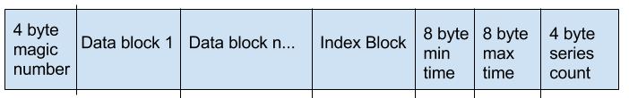
The magic number at the beginning identifies the file as a data file for the PD1 storage engine. We’ll go into the details of the data and index blocks in a bit. The min time and max time are nanosecond epochs of the minimum and maximum timestamps of the points in any of the data blocks of the file. Finally, the file ends with a uint32 of the number of series contained in the data file.

The structure of each data block looks like this:

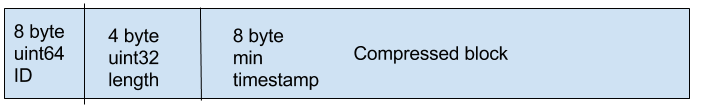
The ID is the identifier for the series and field. IDs are generated by taking the fnv64-a hash of the series key (measurement name + tagset) and the field name. We’ll discuss how we handle ID hash collisions later in this doc.

The compressed block uses a compression scheme depending on the type of the field. Details on compression are covered later, but for now it’s important to know that the first 8 bytes of every compressed block has the minimum timestamp for all values in the block. By default, up to 1000 values are encoded in a block.

The data blocks are always arranged in sorted order by the IDs and if there are multiple blocks for a given ID in a single file, those blocks will be arranged by time. The timestamps for values in the blocks for the same ID are increasing and non-overlapping.

The index block in a data file looks like this:

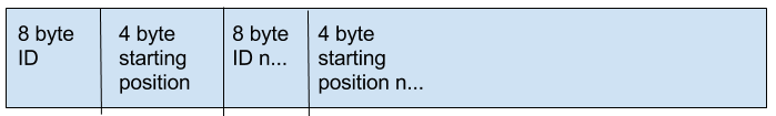
The index block contains all the IDs that have data blocks in the file and the position of their first block. All IDs are in sorted order, which is important later for finding the starting position of an ID’s block. Note that the starting position is a uint32 value, which means that data files are limited in size to a maximum of 4GB.

Writes to the Index

The storage index keeps a collection of data files. These files have non-overlapping time ranges. The index keeps a mapping in memory of the memory mapped data files that exist and their min and max times. The files are kept in a sorted array by their time.

The first thing that happens when the WAL flushes a block of writes to the index is mapping the keys of the series and fields that have values to their unique ID. Most IDs should simply be the fnv64-a hash of the series key and the field name. However, we need to ensure that we keep track of any collisions.

The index keeps a file called “names” that keeps a compressed JSON map of key to ID. When a flush happens we ensure that any of the keys coming in have an ID in the map that is equal to the fnv64-a hash. If it is present in the map and the same we move on. If it isn’t present in the map, we add it. If the ID is taken already, we keep track of the collision.

If there are any new keys, we marshall, compress and write a new names file. The old file is removed once the new one has been written and closed. If there are any collisions, we write those into a collisions file. This is read on startup of the index so collisions can be kept in memory. We’ll talk more about how collisions are handled later.

This name decoding scheme is fairly inefficient since we’re marshaling this entire map on every WAL flush. The alternative is to keep it in memory, but that is also expensive as there are many indexes (one per shard) in a running InfluxDB process. We could also just keep the map in memory while a given shard is hot for writes (i.e. its time range is current for now).

In testing the cost of decoding and rewriting the names file hasn’t been a big problem and the simplicity of the scheme makes it a bit easier to work with. We’ve been testing up to 500k unique keys at this point.

After the ID resolution is done the write will be broken up by the time of the individual data points. If no data file exists for any of the time ranges, a new one will be created and written. If a data file already exists for the given time range and it is less than a configurable size (5MB by default), then the data file will be read in and the new values merged with it and a new data file will be created.

While this new file is getting written, all queries will hit the old data file and continue to use the WAL cache, which won’t be cleared until the write to the index is confirmed. Once the new file is written, the engine will obtain a write lock to replace the old data file with the new data file in the in memory index, remove the old file from the filesystem and then return success back to the WAL. We’ll talk about how recovery is handled in a later section of this document.

Because of this structure, multiple ranges of time can be written simultaneously, which enables us to perform compactions on old time ranges while still accepting writes for current time ranges. We’ll cover the details of compaction in a later section. Writes will only block reads during the window of time that the in-memory sorted list of data files is modified (an operation that takes less than a few microseconds).

The index is optimized for the append only workload that is most common in InfluxDB usage. It’s possible to update old data points, but that operation can be expensive because data files will need to be rewritten. However, historical backfill when initially setting up a database is very efficient and has a workload that looks like filling in new data as long as the backfill is done in time ascending order.

Even during normal operation, data files continually get rewritten as the WAL flushes to the index. However, the data files are generally small at that point so the cost of rewriting them is negligible. Later, compactions will combine older data files into larger ones.

Compaction

In the background the index continually checks for old data files that can be combined together. By default, any files with a time older than 30 minutes will be combined together. The process is the same as during a write, a new file is created, the two data files are read in together and the merged stream of sorted IDs and blocks are written out as they are read from the two files.

Once the new file is written, the index obtains the write lock to modify the collection of data files and removes the older two files. The compaction process will only attempt to compact data files that are less than a configurable size (500MB by default and up to a max of 1GB).

Updates

Updates are held first in the WAL. If there are a number of updates to the same range, ideally the WAL will buffer them together before it gets flushed to the index. The index will simply rewrite the data file that contains the updated data. If the updates are to a recent block of time, the updates will be relatively inexpensive.

Deletes

Deletes are handled in two phases. First, when the WAL gets a delete it will persist it in the log, clear its cache of that series, and tell the index to keep an in-memory tombstone of the delete. When a query comes into the index, it will check it against any of the in-memory tombstones and act accordingly.

Later, when the WAL flushes to the index, it will include the delete and any data points that came into the series after the delete. The index will handle the delete first by rewriting any data files that contain that series to remove them. Then it will persist any new data (for this series or any others), remove the tombstone from memory and return success to the WAL.

Metadata

Metadata for all the series and fields in the shard are kept in 2 files named “names” and “fields”. These two files contain a single Snappy compressed block of the serialized JSON of any names or fields in the shard.

This means that any flush from the WAL that contains either new fields or series, will force the old file to be read in, decompressed, marshalled, merged with the new series and a new file to be written. Because the WAL buffers these new definitions, the cost is generally negligible. However, as the number of series in a shard gets very high it can become expensive. We’ve tested up to 500k unique series and this scheme still works well.

Seeking and Reading a Series

When a seek comes into the storage engine, it is a seek to a given time associated with a specific series key and field. First, we do a binary search on the data files to find the file that has a time range that matches the time we’re seeking to.

Once we have the data file we need to find the position in the file for the block that contains the given time. First, we check the collisions map to see if this seek is to an ID that doesn’t match up with the hash ID. If it’s not there, we do a fnv64-a hash against the series key and field name to get its ID.

Now that we have the ID we check the end of the file for the series count. Remember that it’s memory mapped so this should be fast. Now that we know the count of the series, we know which byte positions in the file contain the index of IDs to starting position.

We’ll now do a binary search against the section of the index to find the ID and its position. Remember that the index is sorted by increasing IDs. This operation is very efficient and the index for a data file is in the memory map.

Now that we have the starting position we can look at the first block’s timestamp and the next block’s timestamp. We traverse the blocks until we find the one that matches up with the timestamp we’re seeking to. This means we’re making jumps in the file by the length of the compressed blocks.

In practice, a shard will have the data for a day or 7 days. For people with regular time series that sample every 10 seconds, they’ll have data files that contain either 8,640 data points (1 day) for each series or that times 7. That means that at most we’ll end up making 56 jumps to the last block. In practice it’s likely that 7 days of data would be split across multiple data files, reducing the number of blocks for a given series in a file.

Once we’ve found the matching block, we decompress it and go to the specific point. As the query engine traverses the series by getting subsequent points, we go through that block, then decompress the next one, then jump to the next data file, until we ultimately reach the end of the shard.

Compression

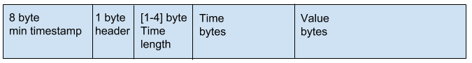
Each block is compressed to reduce storage space and disk IO when querying. A block contains the timestamps and values for a given series and field. Each block has one byte header, followed by the compressed timestamps and then the compressed values. The timestamps and values are stored separately as two compressed parts using different encodings depending on the data type and its shape. Storing them independently allows timestamp encoding to be used with different field types more easily. It also allows for different encodings to be used depending on the type of the data. For example, some points may be able to use run-length encoding whereas other may not. Each value type also contains a 1 byte header indicating the type of compression for the remaining bytes. The four high bits store the compression type and the four low bits are used by the encoder if needed.

Timestamp encoding is adaptive and based on the structure of the timestamps that are encoded. It uses a combination of delta encoding, scaling and compression using simple8b, run-length encoding as well as falling back to no compression if needed.

Timestamp resolution can be as granular as a nanosecond and, uncompressed, require 8 bytes to store. During encoding, the values are first delta-encoded. The first value is the starting timestamp and subsequent values are the differences from the prior value. This usually converts the values into much smaller integers that are easier to compress. Many timestamps are also monotonically increasing and fall on even boundaries of time such as every 10s. When timestamps have this structure, they are scaled by the largest common divisor that Zis also a factor of 10. This has the effect of converting very large integer deltas into smaller ones that compress even better.

Using these adjusted values, if all the deltas are the same, the time range is stored using run-length encoding. If run-length encoding is not possible and all values are less than 1 << 60 - 1 (~36.5 yrs in nanosecond resolution), then the timestamps are encoded using the simple8b encoding which is a 64bit word-aligned integer encoding. This encoding packs up multiple integers into a single 64bit word. If any value exceeds the maximum values, the deltas are stored uncompressed using 8 bytes each for the block. Future encodings will use a patched scheme such as Patched Frame-Of-Reference (PFOR) to handle outlier more effectively.

Floats are encoded using an implementation of the Facebook Gorilla paper. This encoding XORs consecutive values together which produces a small result when the values are close together. The delta is then stored using control bits to indicate how many leading and trailing zero are in the XOR value. Our version removes the timestamp encoding, as described in paper, and only encodes the float values.

Integer encoding uses two different strategies depending on the range of values in the uncompressed data. Encoded values are first encoded using zig zag encoding which is also used for signed integers in Google Protocol Buffers. This interleaves positive and negative integers across a range of positive integers.

For example, [-2,-1,0,1] becomes [3,1,0,2]. See https://developers.google.com/protocol-buffers/docs/encoding#signed-integers for more information.

If all the zig zag encoded values less than 1 << 60 - 1, they are compressed using the simple8b encoding. If any values is larger than the maximum value, then values are stored uncompressed in the block.

Booleans are encoded using a simple bit packing strategy where each boolean uses 1 bit. The number of booleans encoded is stored using variable-byte encoding at the beginning of the block.

Strings are encoding using Snappy compression. Each string is packed next each other in order and compressed as one larger block.